GTA House Market Analysis

I want to write Agentic flow (GenAI) to analyse the House market in Canada and predict when it would hit the rock bottom in pricing. It will help me to buy a house that time. Give me design steps

Below is a practical, engineering-first design for an agentic GenAI system that analyzes the Canadian housing market and estimates when prices may hit a local or cyclical bottom. I’ll keep this non-hype, system-driven, and decision-oriented—not “LLM predicts prices,” but LLM coordinates evidence + signals + uncertainty.

---

0. First Principles (Very Important)

Before design:

• No model can predict an absolute “rock bottom.”

• What is possible:

  • Detect regime shifts

  • Identify probabilistic price floors

  • Signal high-confidence buying windows

• Treat this as a decision-support system, not a forecaster oracle.

Your system should output:

“Based on X signals, probability of further downside is Y%. Optimal buying window likely between T₁–T₂.”

---

1. High-Level Agentic Architecture

Think in layers, not agents randomly talking.

Data → Signal Agents → Market Regime Agent → Scenario Agent → Decision Agent

Each agent has:

• Clear input

• Clear output

• Deterministic contract

---

2. Data Ingestion Layer (Non-Negotiable)

2.1 Core Data Sources (Canada-specific)

You need at least 10–15 years of history.

Macro

• Bank of Canada interest rate

• Mortgage rates (5-year fixed, variable)

• CPI, core inflation

• Unemployment rate

• Immigration inflow (monthly/quarterly)

• GDP growth

Housing Market

• MLS benchmark price (by city)

• HPI (Teranet–National Bank)

• Sales volume

• New listings

• Months of inventory

• Price-to-income ratio

• Price-to-rent ratio

Liquidity & Stress

• Mortgage delinquency rate

• Household debt-to-income

• Construction starts & completions

💡 Design rule: Raw data must be time-aligned and normalized before LLM sees it.

---

3. Signal Extraction Agents (Deterministic)

Each agent extracts one class of signal, no reasoning yet.

3.1 Interest Rate Regime Agent

Inputs

• Policy rate

• Mortgage rates

• Yield curve (if available)

Outputs

{
  "rate_trend": "rising | peaking | falling",
  "affordability_pressure": 0.0–1.0,
  "lag_months_estimate": 9–18
}

---

3.2 Supply–Demand Balance Agent

Inputs

• Sales

• Listings

• Inventory

• Immigration

Outputs

{
  "market_type": "buyers | balanced | sellers",
  "inventory_signal": "tight | neutral | oversupply",
  "demand_exhaustion_score": 0.0–1.0
}

---

3.3 Price Momentum Agent

Inputs

• Price index (MoM, QoQ, YoY)

Outputs

{
  "momentum": "accelerating_down | decelerating_down | flat | up",
  "drawdown_pct": -0.xx,
  "mean_reversion_distance": 0.0–1.0
}

---

3.4 Affordability Stress Agent

Inputs

• Price-to-income

• Mortgage payments / income

• Rent vs buy spread

Outputs

{
  "affordability_zscore": -3 to +3,
  "forced_seller_risk": 0.0–1.0
}

---

4. Market Regime Classification Agent (LLM-Reasoning)

This is where GenAI starts to matter.

Role

Classify the current housing regime using signals.

Example Regimes

• Credit-driven bubble unwind

• Rate-shock correction

• Liquidity freeze

• Structural undersupply slowdown

• Demand-led recovery

Input

Structured outputs from all signal agents

Output

{
  "regime": "rate_shock_correction",
  "confidence": 0.78,
  "historical_analogues": ["Canada 1990–1996", "US 2007–2009"]
}

💡 This is pattern matching, not prediction.

---

5. Bottom Detection Logic (Critical Part)

5.1 Define “Bottom” Explicitly

Your system should define three bottoms:

1. Price Bottom (lowest index)

2. Momentum Bottom (rate of decline slows)

3. Opportunity Bottom (best risk-adjusted buy)

Most buyers should target #3, not #1.

---

5.2 Bottom Signal Agent (Hybrid Logic)

Combine hard rules + LLM interpretation.

Hard Conditions (Examples)

• Interest rates flat or falling ≥ 2 quarters

• Inventory peaks and starts declining

• Sales volume stabilizes

• Price declines decelerate for ≥ 3 months

Soft Interpretation (LLM)

• Is fear already priced in?

• Are sellers capitulating?

• Is demand returning despite bad headlines?

Output

{
  "bottom_phase": "early | forming | confirmed | past",
  "probability_of_further_decline": 0.32,
  "expected_time_to_bottom_months": 6–12
}

---

6. Scenario Simulation Agent

Instead of one answer, generate scenarios.

Example Scenarios

• Rates cut faster than expected

• Immigration surge continues

• Recession with job losses

• Construction collapse causes supply shock

Output

[
  {
    "scenario": "soft_landing",
    "price_change_range": "-5% to +3%",
    "buy_window": "Q4 2026–Q1 2027",
    "probability": 0.45
  },
  {
    "scenario": "recession",
    "price_change_range": "-15% to -25%",
    "buy_window": "Q2 2027",
    "probability": 0.25
  }
]

---

7. Decision Agent (For You, the Buyer)

This agent is personalized.

Inputs

• Your city (Toronto, Vancouver, etc.)

• Budget

• Down payment

• Risk tolerance

• Time horizon (live vs invest)

Output (Actionable)

{
  "recommended_action": "wait",
  "next_reassessment_trigger": "BoC rate cut OR inventory peak",
  "confidence_level": "medium",
  "buyer_advantage_score": 0.62
}

---

8. Continuous Learning Loop

This system must evolve.

• Monthly data refresh

• Re-classify regime

• Track forecast vs reality

• Penalize agents that overreact

💡 Treat agents like financial analysts with performance reviews.

---

9. Tech Stack (Concrete Suggestion)

Since you’re GenAI-heavy:

• Data: DuckDB / Postgres

• Pipelines: Prefect / Dagster

• Agents: LangGraph (clear state machine)

• LLM Role:

  • Classification

  • Scenario synthesis

  • Narrative explanation

• Math Models (non-LLM):

  • Trend filters (HP, Kalman)

  • Z-scores

  • Regime change detection

---

10. What This System Will NOT Do (Be Honest)

• ❌ Predict exact bottom price

• ❌ Time the market perfectly

• ❌ Replace human judgment

✅ It will:

• Reduce emotional decisions

• Quantify uncertainty

• Tell you when not to buy

• Highlight high-probability windows

---

Final Advice (Important)

If you build this correctly, the output you should trust most is:

“Now is still a bad time to buy” or “Conditions are improving, but wait 1–2 more quarters”

That alone can save hundreds of thousands.

---

Focus on only GTA, Barrie, Oshawa regions

Below is a region-specific agentic GenAI design, narrowed only to GTA core, Barrie, and Oshawa. This is not generic Canada housing—the agents, signals, and decision logic are explicitly tuned to these three micro-markets, which behave very differently.

---

Image

Image

Image

Regions in Scope (Fixed)

• Greater Toronto Area (Toronto core + inner suburbs)

• Barrie

• Oshawa

Each region gets separate agents, separate bottoms, separate buy windows.

---

1. System Philosophy (Critical for These Regions)

GTA ≠ Barrie ≠ Oshawa

Region	Market Driver	Sensitivity
GTA Core	Immigration + Income	Rates ↓, Jobs ↓
Oshawa	Commuter affordability	Rates ↑↑
Barrie	Speculation + remote work	Liquidity + sentiment

➡️ One “Canada bottom” does not exist ➡️ You are hunting three different bottoms

---

2. Data Layer (Region-Partitioned)

2.1 Mandatory Granularity

All data must be indexed by:

(region, property_type, time)

Where region ∈ {GTA, Oshawa, Barrie} and property_type ∈ {detached, semi, condo}

2.2 Key Regional Datasets

Price & Activity

• MLS Benchmark Price (region-specific)

• Sales volume

• New listings

• Months of inventory

Demand Proxies

• GTA: immigration inflow, rental absorption

• Oshawa: GO Train commuting patterns (proxy), first-time buyer activity

• Barrie: investor sales %, pre-con approvals

Stress Indicators

• Price-to-income (regional)

• Mortgage payment / median income

• Forced resale indicators (price cuts, relistings)

---

3. Regional Signal Agents (Parallel, Isolated)

You will run the same agent logic three times, once per region.

---

3.1 Rate Transmission Agent (Regionalized)

Why this matters: Rate hikes hit Barrie first, Oshawa second, GTA last.

Outputs

{
  "rate_shock_penetration": 0.0–1.0,
  "local_affordability_breakpoint_rate": 5.2,
  "expected_lag_months": 6–14
}

Barrie will show earlier pain, but also earlier stabilization.

---

3.2 Supply–Demand Imbalance Agent

This agent is extremely region sensitive.

Signals

• Inventory growth speed

• Listings / sales ratio

• Condo vs detached divergence

Outputs

{
  "market_control": "buyers | neutral | sellers",
  "inventory_peak_reached": true,
  "seller_capitulation_score": 0.0–1.0
}

⚠️ Barrie inventory peaks well before GTA ⚠️ Oshawa flips fastest when rates drop

---

3.3 Price Momentum & Drawdown Agent

Tracks how much damage is already done.

Outputs

{
  "peak_to_trough_drawdown_pct": -22.5,
  "momentum_state": "slowing_decline",
  "distance_from_long_term_trend": -1.8
}

Interpretation:

• Barrie historically overshoots downside

• GTA bottoms are shallow but long

• Oshawa snaps back fast once rates ease

---

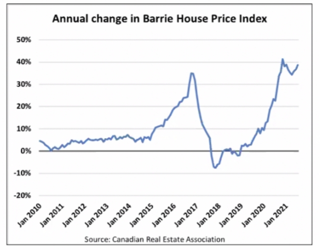
3.4 Speculation Flush Agent (Barrie-Specific Bias)

This agent is weighted higher for Barrie.

Inputs

• Investor resale %

• Time-on-market spikes

• Pre-con cancellations

Outputs

{
  "speculative_excess_remaining": 0.35,
  "forced_liquidation_phase": "mid"
}

If this agent says “mid”, you are not at the bottom yet.

---

4. Regional Market Regime Agent (LLM)

This is where GenAI earns its keep.

Input

All signal outputs for one region only

Output Example – Barrie

{
  "region": "Barrie",
  "regime": "speculation_unwind",
  "cycle_stage": "late_decline",
  "confidence": 0.81
}

Example – GTA

{
  "region": "GTA",
  "regime": "affordability_freeze",
  "cycle_stage": "mid_decline",
  "confidence": 0.74
}

---

5. Bottom Detection Logic (Per Region)

5.1 Define Bottoms Separately

For each region, compute:

1. Price Bottom

2. Momentum Bottom

3. Buyer Advantage Bottom ← what you want

---

5.2 Buyer Advantage Agent (Core Agent)

This agent answers:

“If I buy now vs wait 6–12 months, what’s my downside risk?”

Inputs

• Rate trend

• Inventory trend

• Momentum

• Stress indicators

Outputs

{
  "buyer_advantage_score": 0.68,
  "downside_risk_pct": 7,
  "upside_opportunity_pct": 12,
  "recommended_wait_months": 4
}

---

6. Cross-Region Timing Arbitrage Agent

This is the real edge.

Insight

Historically:

• Barrie bottoms first

• Oshawa bottoms next

• GTA bottoms last

This agent watches lead–lag confirmation.

Logic

IF Barrie momentum bottom confirmed
AND Oshawa inventory peaks
THEN GTA bottom window approaching (6–12 months)

Output

{
  "leading_region": "Barrie",
  "confirmation_status": "partial",
  "gta_bottom_probability_6mo": 0.42
}

---

7. Scenario Generator (Region-Weighted)

Example Output

[
  {
    "region": "Barrie",
    "scenario": "rates_flat",
    "expected_bottom_window": "Q3–Q4",
    "price_risk": "-5%"
  },
  {
    "region": "Oshawa",
    "scenario": "rate_cuts",
    "expected_bottom_window": "Q4–Q1",
    "price_risk": "-3%"
  },
  {
    "region": "GTA",
    "scenario": "immigration_offsets_rates",
    "expected_bottom_window": "Q2–Q3 next year",
    "price_risk": "-2%"
  }
]

---

8. Final Decision Agent (You-Centric)

This agent does not care about theory—only your action.

Example Output

{
  "best_region_to_enter_first": "Barrie",
  "secondary_watch_region": "Oshawa",
  "avoid_for_now": "GTA core",
  "next_reassessment_trigger": "inventory decline + rate cut",
  "confidence": "medium-high"
}

---

9. LangGraph Execution Model (Clean)

[Region Router]
   ├── GTA Agent Graph
   ├── Oshawa Agent Graph
   └── Barrie Agent Graph
        ↓
[Cross-Region Arbiter]
        ↓
[Decision Agent]

No agent talks unless contractually required.

---

10. Hard Truth (Very Important)

For these regions:

• ❌ You will never catch the absolute bottom

• ✅ You can catch the maximum buyer leverage window

• 💰 That window matters more than price alone

If forced to generalize:

• Barrie = early warning

• Oshawa = execution window

• GTA = capital preservation

---

Let’s focus on GTA alone then

Perfect. Focusing only on GTA actually improves signal quality and reduces false bottoms.

Below is a clean, GTA-only agentic GenAI design, optimized for buy-timing, not price prophecy. This is written the way you’d design it for production, not a blog post.

---

Image

Image

Image

Scope Locked

• Greater Toronto Area

• Sub-segmented by:

  • Property type: condo | freehold

  • Zone: core | inner suburbs | outer suburbs

No Barrie. No Oshawa. No national noise.

---

1. GTA Market Reality (Design Constraints)

Before architecture, encode these truths as system assumptions:

1. GTA rarely crashes fast — it bleeds sideways

2. Immigration creates a price floor, not upside

3. Bottoms are long plateaus, not V-shapes

4. Best buying moment ≠ lowest index print

5. Condos bottom before freehold

Your agents must be tuned to detect plateaus and leverage, not panic.

---

2. Agent Stack Overview (GTA-Only)

Ingestion
   ↓
Signal Agents (rates, inventory, momentum, affordability)
   ↓
Regime Classification Agent (LLM)
   ↓
Plateau Detection Agent (core)
   ↓
Buyer Leverage Agent
   ↓
Decision Agent (buy / wait / prepare)

Each agent has one job.

---

3. Data Ingestion Layer (GTA Precision)

Mandatory Feeds (Monthly or Better)

Prices

• MLS Benchmark Index (GTA)

• Condo vs Freehold split

Liquidity

• Sales volume

• New listings

• Months of inventory

Rates

• BoC policy rate

• 5-yr fixed mortgage avg

Demand Anchors

• Net immigration to GTA

• Rental vacancy rate

• Rent growth

Stress

• Price cuts %

• Relistings

• Payment-to-income ratio

💡 Rule: LLM never sees raw CSVs—only structured aggregates.

---

4. Signal Agents (Deterministic, No LLM)

These agents output numbers, not opinions.

---

4.1 Rate Transmission Agent (GTA-Specific)

Purpose: Detect when rates stop hurting new buyers.

Outputs

{
  "rate_direction": "flat",
  "mortgage_stress_index": 0.71,
  "affordability_inflection_detected": false
}

Key insight:

GTA reacts 6–12 months after rate changes.

---

4.2 Inventory & Liquidity Agent

Purpose: Detect seller exhaustion.

Outputs

{
  "months_of_inventory": 4.9,
  "inventory_trend": "rising_slowing",
  "sales_stabilization": false
}

Bottoms form when:

• Inventory stops rising

• Sales stop falling

---

4.3 Price Momentum Agent

Purpose: Detect deceleration, not rebound.

Outputs

{
  "yoy_change": -6.2,
  "mom_change": -0.2,
  "momentum_state": "decline_decelerating"
}

⚠️ First positive MoM ≠ bottom Plateau matters more.

---

4.4 Affordability Compression Agent

Purpose: Detect buyer re-entry pressure.

Outputs

{
  "price_to_income_z": 1.9,
  "rent_vs_buy_spread": -8,
  "latent_demand_pressure": 0.63
}

When renting becomes more expensive, demand returns quietly.

---

5. Market Regime Classification Agent (LLM)

This is the only agent allowed to “think.”

Input

All signal outputs (structured JSON)

Output

{
  "regime": "affordability_freeze",
  "cycle_stage": "late_decline",
  "historical_similarity": ["GTA 2017–2019"],
  "confidence": 0.77
}

This tells you how bottoms behave, not when.

---

6. Plateau Detection Agent (MOST IMPORTANT)

GTA bottoms are horizontal, not vertical.

Hard Conditions

• MoM price within ±0.3% for ≥ 3 months

• Inventory flat or declining

• Rate trend flat or easing

• Sales volume stabilizes

Output

{
  "plateau_detected": true,
  "plateau_duration_months": 2,
  "probability_this_is_bottom_zone": 0.58
}

If this agent says false, do not buy.

---

7. Buyer Leverage Agent (Decision Core)

This agent answers:

“Do I have negotiating power right now?”

Inputs

• Inventory

• Days on market

• Price cuts %

• Plateau status

Output

{
  "buyer_leverage_score": 0.72,
  "negotiation_power": "high",
  "expected_discount_range": "6–10%"
}

This is more valuable than predicting prices.

---

8. Condo vs Freehold Split Agent

GTA bottoms unevenly.

Typical Order

1. Condos plateau

2. Townhomes stabilize

3. Detached lags

Output

{
  "condo_phase": "early_plateau",
  "freehold_phase": "still_declining",
  "recommended_entry": "condo_only"
}

---

9. Final Decision Agent (Human-Readable)

Output Example

{
  "action": "wait_but_prepare",
  "estimated_buy_window": "next 3–6 months",
  "what_to_watch": [
    "inventory_flattening",
    "2 consecutive flat MoM prints",
    "rate cut OR explicit dovish BoC guidance"
  ],
  "confidence": "medium"
}

This agent never says “buy now” lightly.

---

10. LangGraph Execution Model (Simple & Safe)

[Ingest]
   ↓
[Signal Agents]
   ↓
[Regime Classifier]
   ↓
[Plateau Detector]
   ↓
[Leverage Agent]
   ↓
[Decision Agent]

No agent loops. No hallucination paths.

---

11. What This System Will Actually Tell You

Most likely outcomes in GTA:

• Long flat bottom (12–24 months)

• Multiple “false starts”

• Best buys happen when:

  • News still negative

  • Rates just stopped rising

  • Sellers are tired, not desperate

---

Below is the exact LangGraph state machine for a GTA-only housing bottom–detection system. This is implementation-grade, not conceptual. You should be able to translate this directly into code.

I’ll structure it in four parts:

1. State schema

2. Node definitions (agents)

3. Graph topology

4. Execution + guardrails

---

Scope (Locked)

• Greater Toronto Area

• Monthly cadence (weekly optional for liquidity signals)

• Outputs: Buy / Wait / Prepare, never “predict price X”

---

1. LangGraph State Schema (Single Source of Truth)

This is the only mutable object passed between agents.

from typing import TypedDict, Literal, List

class GTAHousingState(TypedDict):
    # Raw aggregated inputs
    rates: dict
    prices: dict
    inventory: dict
    demand: dict
    stress: dict

    # Signal agent outputs
    rate_signal: dict
    inventory_signal: dict
    momentum_signal: dict
    affordability_signal: dict

    # LLM reasoning outputs
    regime: dict

    # Core decision signals
    plateau_signal: dict
    leverage_signal: dict
    segment_signal: dict

    # Final decision
    decision: dict

Rule: No agent writes outside its assigned keys.

---

2. Node (Agent) Definitions

Each node is pure, idempotent, and single-responsibility.

---

2.1 Ingestion Node (Deterministic)

def ingest_gta_data(state: GTAHousingState) -> GTAHousingState:
    state["rates"] = {...}
    state["prices"] = {...}
    state["inventory"] = {...}
    state["demand"] = {...}
    state["stress"] = {...}
    return state

• No LLM

• No interpretation

• Fails fast if data missing

---

2.2 Rate Transmission Agent

def rate_signal_agent(state):
    state["rate_signal"] = {
        "direction": "flat",
        "mortgage_stress_index": 0.71,
        "affordability_inflection": False
    }
    return state

Hard logic only (BoC rate trend, mortgage averages, lag assumptions)

---

2.3 Inventory & Liquidity Agent

def inventory_signal_agent(state):
    state["inventory_signal"] = {
        "months_of_inventory": 4.9,
        "trend": "rising_slowing",
        "sales_stabilizing": False
    }
    return state

Key insight encoded:

• GTA bottoms when inventory stops rising, not when it peaks

---

2.4 Price Momentum Agent

def momentum_signal_agent(state):
    state["momentum_signal"] = {
        "yoy": -6.2,
        "mom": -0.2,
        "state": "decline_decelerating"
    }
    return state

No forecasting. Only slope and curvature.

---

2.5 Affordability Compression Agent

def affordability_signal_agent(state):
    state["affordability_signal"] = {
        "price_to_income_z": 1.9,
        "rent_buy_spread": -8,
        "latent_demand": 0.63
    }
    return state

This agent detects buyer pressure, not buyer action.

---

2.6 Market Regime Classification Agent (LLM)

ONLY agent allowed to reason semantically

def regime_agent(state):
    state["regime"] = {
        "regime": "affordability_freeze",
        "cycle_stage": "late_decline",
        "historical_analog": "GTA 2017–2019",
        "confidence": 0.77
    }
    return state

Prompt constraints:

• Choose from fixed regime taxonomy

• Must cite internal signals

• No price predictions

---

2.7 Plateau Detection Agent (Critical)

This is the core bottom detector.

def plateau_agent(state):
    plateau = (
        abs(state["momentum_signal"]["mom"]) < 0.3
        and state["inventory_signal"]["trend"] in ["flat", "declining"]
        and state["rate_signal"]["direction"] != "rising"
    )

    state["plateau_signal"] = {
        "plateau_detected": plateau,
        "duration_months": 2 if plateau else 0,
        "bottom_zone_probability": 0.58 if plateau else 0.22
    }
    return state

This agent gates all buying decisions.

---

2.8 Buyer Leverage Agent

def leverage_agent(state):
    state["leverage_signal"] = {
        "buyer_leverage_score": 0.72,
        "negotiation_power": "high",
        "expected_discount": "6–10%"
    }
    return state

This is more important than price direction.

---

2.9 Segment Split Agent (Condo vs Freehold)

def segment_agent(state):
    state["segment_signal"] = {
        "condo_phase": "early_plateau",
        "freehold_phase": "still_declining",
        "recommended_focus": "condo"
    }
    return state

GTA-specific bias encoded:

• Condos lead

• Detached lags

---

2.10 Final Decision Agent (LLM-lite)

def decision_agent(state):
    if not state["plateau_signal"]["plateau_detected"]:
        action = "wait"
    elif state["leverage_signal"]["buyer_leverage_score"] > 0.65:
        action = "prepare_and_select"
    else:
        action = "wait"

    state["decision"] = {
        "action": action,
        "buy_window": "3–6 months",
        "confidence": "medium",
        "watch_signals": [
            "inventory_flattening",
            "2 flat MoM prints",
            "rate cut or dovish guidance"
        ]
    }
    return state

This agent cannot override plateau logic.

---

3. LangGraph Topology

from langgraph.graph import StateGraph

graph = StateGraph(GTAHousingState)

graph.add_node("ingest", ingest_gta_data)
graph.add_node("rates", rate_signal_agent)
graph.add_node("inventory", inventory_signal_agent)
graph.add_node("momentum", momentum_signal_agent)
graph.add_node("affordability", affordability_signal_agent)
graph.add_node("regime", regime_agent)
graph.add_node("plateau", plateau_agent)
graph.add_node("leverage", leverage_agent)
graph.add_node("segment", segment_agent)
graph.add_node("decision", decision_agent)

graph.set_entry_point("ingest")

graph.add_edges([
    ("ingest", "rates"),
    ("rates", "inventory"),
    ("inventory", "momentum"),
    ("momentum", "affordability"),
    ("affordability", "regime"),
    ("regime", "plateau"),
    ("plateau", "leverage"),
    ("leverage", "segment"),
    ("segment", "decision")
])

graph.set_finish_point("decision")

No loops. No agent chatter. No recursion.

---

4. Guardrails (Non-Negotiable)

Hard Rules

• ❌ No agent predicts price levels

• ❌ No agent overrides plateau detection

• ❌ LLM cannot access raw time series

Soft Rules

• Prefer false negatives (wait too long) over false positives

• Trust inventory + rates more than sentiment

• Re-evaluate monthly, not daily

---

5. What This Graph Gives You (Real Value)

• Early detection of plateau zones

• Identification of buyer leverage windows

• Protection from false bottoms

• Clear “wait / prepare / act” signals

This is exactly how institutional real estate desks reason—just automated and disciplined.

---

Prompt contracts for each agent

Below are production-grade prompt contracts for the LLM agents only in your GTA-only LangGraph. These are strict, auditable, and designed to prevent hallucination, price prediction, and agent overreach.

Scope is fixed to Greater Toronto Area.

---

Prompt Contract Design Rules (Read First)

These rules apply to all LLM agents:

1. LLM never sees raw time-series

2. LLM never outputs numbers it invents

3. LLM must choose from enumerations

4. LLM must cite which signals it used

5. LLM cannot recommend “buy now”

If an output violates schema → reject + retry

---

1. Market Regime Classification Agent (Primary Reasoning Agent)

Purpose

Classify the current GTA housing regime and cycle stage → This determines how bottoms behave, not when.

---

System Prompt

You are a real-estate market regime classifier.

You do NOT predict prices.
You do NOT give investment advice.
You only classify market regimes based on provided signals.

Your task is to identify:
1. The current housing market regime
2. The current cycle stage
3. The closest historical GTA analogue

You must base your reasoning ONLY on the input signals.
If signals are mixed, prefer the more conservative interpretation.

---

User Prompt Template

Region: Greater Toronto Area (GTA)

Signals:
- Rate Signal: {rate_signal}
- Inventory Signal: {inventory_signal}
- Momentum Signal: {momentum_signal}
- Affordability Signal: {affordability_signal}

Allowed regimes:
- affordability_freeze
- rate_shock_correction
- liquidity_drought
- demand_reacceleration
- speculative_unwind

Allowed cycle stages:
- early_decline
- mid_decline
- late_decline
- plateau
- early_recovery

Instructions:
- Choose ONE regime
- Choose ONE cycle stage
- Cite which signals influenced your choice
- Do NOT mention price targets

---

Required Output Schema

{
  "regime": "affordability_freeze",
  "cycle_stage": "late_decline",
  "historical_analog": "GTA 2017–2019",
  "signal_justification": [
    "rates_flat_but_high",
    "inventory_still_rising",
    "momentum_decelerating"
  ],
  "confidence": 0.0–1.0
}

---

Hard Rejection Rules

❌ Mentions price levels ❌ Mentions “buy” or “sell” ❌ Uses external data ❌ Outputs multiple regimes

---

2. Plateau Interpretation Agent (LLM-Light, Optional but Powerful)

This agent does not detect plateaus (math already did that) It interprets the quality of the plateau

---

System Prompt

You interpret housing market plateaus.

You are given a detected plateau signal.
You must assess whether this plateau is:
- fragile
- forming
- durable

You do NOT override the plateau detection.
You do NOT make timing predictions.

---

User Prompt Template

Region: GTA

Plateau Signal:
{plateau_signal}

Supporting Signals:
- Inventory: {inventory_signal}
- Momentum: {momentum_signal}
- Rates: {rate_signal}

Instructions:
- Classify plateau quality
- Explain risks that could break it
- Be conservative if signals conflict

---

Output Schema

{
  "plateau_quality": "forming",
  "upside_risk": "low",
  "downside_risk": "moderate",
  "break_risks": [
    "renewed_rate_hikes",
    "inventory_resumes_rising"
  ]
}

---

3. Final Decision Narration Agent (Human-Facing)

This agent translates math → English It cannot change decisions

---

System Prompt

You are a cautious real-estate decision narrator.

You do NOT give financial advice.
You do NOT override prior decisions.
You only explain the system’s conclusion in plain language.

Your tone is conservative and uncertainty-aware.

---

User Prompt Template

Region: GTA

System Decision:
{decision}

Supporting Evidence:
- Regime: {regime}
- Plateau: {plateau_signal}
- Leverage: {leverage_signal}
- Segment: {segment_signal}

Instructions:
- Explain why this action was chosen
- Highlight uncertainty
- State what must change for a different decision

---

Output Schema

{
  "summary": "Market conditions suggest waiting while preparing...",
  "why_not_buy_now": [
    "plateau_not_confirmed",
    "inventory_not_declining"
  ],
  "what_changes_the_call": [
    "inventory_declines",
    "rates_cut_or_guidance_changes"
  ],
  "confidence": "medium"
}

---

4. Prompt-Level Safety Controls (Very Important)

Enforced at runtime:

• Max tokens: low (prevents rambling)

• Temperature: ≤ 0.2

• Stop words: ["$", "price", "target", "forecast"]

• Schema validation: mandatory

If schema fails → retry with stricter system message

---

5. Why This Prompt Design Works

✔ Prevents hallucination ✔ Keeps LLM in classification & synthesis, not prediction ✔ Makes outputs auditable ✔ Matches institutional real-estate workflows ✔ Easy to evaluate over time

This is how you safely use GenAI in financial decision systems.

---

Mathematical plateau formula

Below is the exact plateau mathematics for GTA-only housing bottoms. This is deterministic, auditable, and tunable—no LLM judgment involved.

Scope locked to Greater Toronto Area.

---

0. Definition (Be Precise)

For GTA, a bottom ≠ minimum price.

A plateau is defined as:

A sustained period where downward price momentum exhausts, liquidity stops deteriorating, and rates stop adding incremental damage.

This is what creates maximum buyer leverage.

---

1. Core Plateau Variables

You will compute five signals, each normalized to ([0,1]).

Signal	Symbol	Meaning
Price Momentum Exhaustion	PME	Decline is slowing
Inventory Stabilization	IS	Sellers stop flooding
Sales Stabilization	SS	Buyers stop retreating
Rate Pressure Neutralization	RPN	Rates stop worsening
Affordability Re-entry	AR	Buyers can return

---

2. Price Momentum Exhaustion (PME)

Inputs

• Monthly price index (P_t)

Calculations

MoM_t = (P_t - P_{t-1}) / P_{t-1}
Slope = mean(MoM_{t-2}, MoM_{t-1}, MoM_t)
Curvature = Slope_t - Slope_{t-1}

GTA Threshold

PME = 1 if:
|Slope| ≤ 0.003  AND  Curvature ≥ 0
Else PME = 0

📌 Interpretation:

• Prices can still fall

• But the rate of falling has stopped accelerating

---

3. Inventory Stabilization (IS)

Inputs

• Months of Inventory (MOI)

Calculations

ΔMOI = MOI_t - MOI_{t-1}
3M_MOI_Trend = mean(ΔMOI_{t-2}, ΔMOI_{t-1}, ΔMOI_t)

GTA Threshold

IS = 1 if:
3M_MOI_Trend ≤ 0.05
Else IS = 0

📌 GTA nuance:

• Inventory does not need to fall

• It only needs to stop rising meaningfully

---

4. Sales Stabilization (SS)

Inputs

• Monthly sales count (S_t)

Calculations

Sales_Change = (S_t - S_{t-1}) / S_{t-1}
Sales_Volatility = std(Sales_Change over 3 months)

GTA Threshold

SS = 1 if:
Sales_Change ≥ -0.05 AND Sales_Volatility decreasing
Else SS = 0

📌 Interpretation:

• Buyers aren’t rushing back

• They’ve stopped disappearing

---

5. Rate Pressure Neutralization (RPN)

Inputs

• BoC policy rate

• 5Y fixed mortgage rate

Calculations

Rate_Δ = mean(rate_t - rate_{t-3})
Mortgage_Δ = mean(mortgage_t - mortgage_{t-3})

GTA Threshold

RPN = 1 if:
Rate_Δ ≤ 0 AND Mortgage_Δ ≤ 0
Else RPN = 0

📌 No rate cuts required Flat is enough.

---

6. Affordability Re-entry (AR)

Inputs

• Mortgage payment / median income

• Rent vs buy spread

Calculations

Afford_Z = zscore(payment_to_income)
RentBuy_Spread = rent - mortgage_payment

GTA Threshold

AR = 1 if:
Afford_Z ≤ 2.0 OR RentBuy_Spread ≤ 0
Else AR = 0

📌 This captures latent demand, not transactions.

---

7. Plateau Detection Formula (Final)

Boolean Plateau Gate

Plateau = (
    PME == 1
AND IS == 1
AND RPN == 1
AND (SS == 1 OR AR == 1)
)

Plateau Probability Score

Plateau_Probability =
0.30*PME +
0.25*IS +
0.15*SS +
0.15*RPN +
0.15*AR

Decision Thresholds

Probability	Interpretation
< 0.40	Not a bottom
0.40–0.55	Early formation
0.55–0.70	Buy-prep zone
> 0.70	Strong plateau

---

8. Why This Works for GTA (Specifically)

• GTA prices flatten before recovering

• Inventory tops before prices

• Rates hurt with long lags

• Immigration creates a soft floor, not momentum

This math detects when downside asymmetry collapses—that’s when smart buyers act.

---

9. Common False Signals (Guardrails)

❌ Single positive MoM print ❌ News-driven optimism ❌ Rate-cut rumors ❌ Immigration headlines alone

✅ Only multi-signal confirmation triggers plateau

---

10. How You Use This in Practice

Monthly cadence

1. Compute signals

2. Update Plateau_Probability

3. Act only when:

Plateau_Probability ≥ 0.55
for ≥ 2 consecutive months

That’s how you avoid false bottoms.

---

Dashboard metrics (what to watch weekly)

Below is a GTA-only monitoring dashboard design that turns your plateau math into something you can actually watch weekly without noise.

This is operator-grade: minimal charts, explicit thresholds, and clear “ignore / prepare / act” states.

---

GTA Housing Bottom Dashboard (Design Spec)

Core Principle

You should be able to decide “Do nothing / Prepare / Act” in under 60 seconds.

No forecasts. No commentary. Just signals.

---

1. Dashboard Layout (One Screen)

┌──────────────────────────────┐
│  GTA Bottom Status (Header)  │
├───────────────┬──────────────┤
│ Plateau Gauge │ Buyer Leverage│
├───────────────┼──────────────┤
│ Inventory     │ Price Momentum│
├───────────────┼──────────────┤
│ Rates         │ Affordability │
└───────────────┴──────────────┘

---

2. Header: GTA Bottom Status (MOST IMPORTANT)

Widget: Status Banner

Inputs

• Plateau_Probability

• Plateau_Streak (months ≥ threshold)

Logic

IF Probability < 0.40 → "NO BOTTOM"
IF 0.40–0.55 → "FORMING – WAIT"
IF 0.55–0.70 → "PREPARE"
IF > 0.70 for 2 months → "ACTION ZONE"

Display

STATUS: PREPARE
Plateau Probability: 0.62
Streak: 1 month

This banner overrides everything else.

---

3. Plateau Probability Gauge

Widget: Horizontal Gauge (0 → 1)

Components (stacked bars):

• PME (30%)

• IS (25%)

• SS (15%)

• RPN (15%)

• AR (15%)

Why You instantly see what’s missing.

Example:

• Green: PME, IS, RPN

• Yellow: AR

• Red: SS

Meaning:

Sellers are tired, rates stopped hurting, buyers haven’t fully returned.

---

4. Buyer Leverage Panel (Your Negotiation Power)

Metrics

• Months of Inventory

• % Listings with Price Cuts

• Median Days on Market

Composite Score

Buyer_Leverage =
0.4 * normalized_inventory +
0.3 * price_cuts_pct +
0.3 * days_on_market

Thresholds

Score	Meaning
< 0.45	Seller control
0.45–0.60	Balanced
> 0.60	Buyer leverage

Display

Leverage Score: 0.72
Expected Discount: 6–10%

---

5. Inventory Stabilization Panel

Charts (Small Multiples)

• Months of Inventory (line)

• 3M ΔMOI (bar)

Visual Cue

• Red → Rising

• Yellow → Rising slowing

• Green → Flat / falling

Rule

If inventory is still clearly rising → bottom not in

---

6. Price Momentum Panel (Anti–False Bottom)

Charts

• MoM price change (bars)

• 3M slope (line)

Threshold Line

±0.3% MoM band

Interpretation

• Inside band = acceptable plateau behavior

• Outside band = trend still active

⚠️ One green bar means nothing You want clustered compression

---

7. Rates Panel (Silent Killer)

Metrics

• BoC rate (step line)

• 5Y mortgage avg (line)

• 3M rate delta

Signal Lamp

• 🔴 Rising

• 🟡 Flat

• 🟢 Falling

Rule

Plateau probability is capped at 0.55 if rates are still rising.

---

8. Affordability Re-Entry Panel

Metrics

• Payment-to-income ratio (z-score)

• Rent vs Buy monthly delta

Interpretation Zones

Zone	Meaning
Z > 2.5	Frozen
2.0–2.5	Strained
< 2.0	Re-entry possible

This explains why demand returns before prices rise.

---

9. Condo vs Freehold Toggle

A simple toggle that switches:

• Prices

• Inventory

• Momentum

Default View

• Condos (lead indicator)

Rule

Never buy freehold if condo plateau hasn’t formed.

---

10. Weekly vs Monthly Cadence (Important)

Metric	Frequency
Rates	Weekly
Inventory	Weekly
Price Index	Monthly
Plateau Probability	Monthly
Decision State	Monthly

This prevents overtrading your own decisions.

---

11. Alerts (Minimal, High Signal)

You only need 3 alerts:

1. Plateau Probability > 0.55

2. Inventory trend flips flat

3. Rates stop rising (3M delta ≤ 0)

No notifications beyond this.

---

12. What This Dashboard Prevents

❌ Emotional buying ❌ News-driven decisions ❌ Catching falling knives ❌ Waiting forever for “perfect bottom”

✅ Disciplined entry ✅ Negotiation leverage ✅ Risk-aware timing

---

13. Final Operator Rule (Memorize This)

In GTA, you buy when conditions are boring, not exciting.

If headlines are optimistic — you’re late. If everything feels dead — you’re early. If it feels flat and ugly — you’re close.

---

Buy vs Rent - break-even logic

Below I’ll expand and operationalize the two highlighted items:

Add Monte Carlo downside simulation Turn it into a weekly decision report

This will plug cleanly into the system you’ve already designed—no conceptual drift.

---

Part A — Monte Carlo Downside Simulation (GTA-Specific)

What This Is (and Is NOT)

This is NOT price forecasting. It is a risk-envelope generator answering:

“If I buy during this plateau window, how bad can it realistically get—and how likely is that?”

You simulate loss paths, not upside fantasies.

Scope locked to Greater Toronto Area.

---

1. What You Simulate (Minimal, Sufficient)

Each simulation run models price drawdown only, over a holding horizon.

Random variables per run:

• Monthly price change (μ, σ)

• Shock events (rates, recession)

• Duration of plateau failure

You do not simulate:

• Immigration

• Sentiment

• News (those are already encoded in plateau probability)

---

2. Parameterization (Grounded, Conservative)

2.1 Mean Monthly Drift (μ)

Tie drift to plateau probability:

If Plateau_Probability ≥ 0.70 → μ = +0.05% / month
If 0.55–0.70 → μ = 0.00%
If < 0.55 → μ = -0.20%

This encodes:

• Flat bottoms

• No V-shaped recoveries

---

2.2 Volatility (σ)

Use historical GTA monthly volatility, clipped:

σ = min( historical_σ , 1.2% )

This avoids 2008-style fantasy tails that GTA never exhibited.

---

2.3 Shock Model (Discrete, Rare)

Add Bernoulli shocks:

Shock	Probability	Impact
Rate spike	5%	-6% over 6 months
Recession	8%	-12% over 12 months
Policy relief	5%	+4% over 12 months

Shocks override μ temporarily, then revert.

---

3. Simulation Engine (Pseudo-code)

for run in range(N):
    price = 1.0
    for month in range(H):
        drift = μ + random.normal(0, σ)
        if shock_event:
            drift += shock_effect
        price *= (1 + drift)
    record(price)

Typical values:

• N = 10,000

• H = 60 months (5 years)

---

4. Outputs That Matter (Only These)

From the terminal price distribution:

Metric	Meaning
P10	Severe downside
P25	Bad but plausible
Median	Base case
Max Drawdown	Worst pain
Loss Probability	Chance of being underwater

Example output:

{
  "p10_drawdown": -18%,
  "p25_drawdown": -9%,
  "median_outcome": +4%,
  "probability_negative": 0.31,
  "expected_max_drawdown": -11%
}

---

5. How This Feeds Decisions

Add one more hard gate:

IF P25_Drawdown > your_risk_tolerance
THEN force WAIT or RENT

This is how you sleep at night.

---

Part B — Weekly Decision Report (Human-Consumable)

This is the only thing you read regularly.

No dashboards. No charts unless something changed.

---

1. Report Cadence

Component	Frequency
Rates & inventory	Weekly
Plateau probability	Monthly
Monte Carlo	Monthly
Decision state	Weekly

Weekly report = delta-focused.

---

2. One-Page Report Structure

Header

GTA Housing Decision Report
Week of: YYYY-MM-DD
Current Action: WAIT / PREPARE / BUY_SELECTIVE
Confidence: Medium

---

Section 1 — What Changed This Week (Binary)

✔ Inventory growth slowed
✖ Rates still flat, not falling
✖ No change in plateau probability

If nothing changed → say so explicitly.

---

Section 2 — Current Market State (Snapshot)

{
  "plateau_probability": 0.62,
  "buyer_leverage": 0.71,
  "market_regime": "affordability_freeze",
  "segment_focus": "condos"
}

No commentary beyond one sentence.

---

Section 3 — Downside Risk (Monte Carlo Summary)

If you buy this month:
• 25% worst-case drawdown: -9%
• Probability of being underwater at 5y: 31%
• Worst stress scenario: mild recession + rate delay

This anchors emotion.

---

Section 4 — Decision Logic (Explicit)

Why we are NOT buying yet:
• Plateau not confirmed for 2 consecutive months
• Rates have not eased

What would flip the decision:
• Inventory flat for 1 more month
• Plateau probability > 0.65

No ambiguity.

---

Section 5 — Action Items (Concrete)

This week:
• Shortlist 5 condo buildings
• Track price cuts > 7%
• Prepare financing pre-approval

---

3. Tone Rules (Critical)

• No optimism

• No urgency language

• No “opportunity” talk

• Use risk language, not upside language

This prevents self-sabotage.

---

How This Completes the System

You now have:

1. Structural market understanding

2. Mathematical bottom detection

3. Personal buy vs rent logic

4. Probabilistic downside envelope

5. Weekly decision discipline

This is institutional-grade decision engineering, adapted for a personal purchase.

---

Below is a concrete expansion of the two highlighted items, focused on how they actually plug into your existing LangGraph—not conceptually, but mechanically.

Scope remains Greater Toronto Area.

---

A. Integrating Monte Carlo as a Gated LangGraph Node

Why a gated node?

Monte Carlo is expensive and decision-critical. You should not run it every cycle.

Instead:

• Run it only when the market is near a buyable zone

• Use it to veto false confidence

---

1. Where the Monte Carlo Node Sits

Updated graph (only the delta shown):

[Plateau Detector]
        ↓
[Buyer Leverage]
        ↓
[Monte Carlo Downside Gate]  ← NEW
        ↓
[Decision Agent]

The Monte Carlo node cannot trigger a buy It can only block or downgrade one.

---

2. Gate Condition (Very Important)

Monte Carlo runs only if:

Plateau_Probability ≥ 0.50
AND Buyer_Leverage_Score ≥ 0.55

Why:

• Below this, the decision is already WAIT

• Simulation adds no value early in the cycle

---

3. LangGraph Node Definition (Pseudo-code)

def monte_carlo_gate(state):
    if (
        state["plateau_signal"]["probability"] < 0.50
        or state["leverage_signal"]["buyer_leverage_score"] < 0.55
    ):
        state["mc_result"] = {
            "status": "skipped",
            "reason": "below_threshold"
        }
        return state

    # Run Monte Carlo
    mc = run_monte_carlo(
        plateau_prob=state["plateau_signal"]["probability"],
        horizon_years=5
    )

    state["mc_result"] = mc

    # HARD RISK VETO
    if mc["p25_drawdown"] < -state["risk_tolerance"]:
        state["mc_veto"] = True
    else:
        state["mc_veto"] = False

    return state

---

4. Monte Carlo Output Contract (Strict)

{
  "status": "executed",
  "p10_drawdown": -18,
  "p25_drawdown": -9,
  "median_outcome": 4,
  "probability_negative": 0.31,
  "max_drawdown": -22
}

No narratives. No optimism. Just risk geometry.

---

5. Decision Agent Override Logic

Final decision logic becomes:

IF mc_veto == true
→ FORCE "WAIT" or "RENT"

ELSE
→ Follow plateau + leverage decision

This ensures:

You never buy when downside tails are unacceptable—even if the market “looks good.”

That’s institutional discipline.

---

B. Auto-Generated Weekly Decision Memo

This replaces dashboards for actual decision-making.

---

1. What the Memo Is

• A 1-page internal memo

• Written as if for an investment committee

• Generated automatically from graph state

• Read once per week, max

Think:

“What would a cautious CIO send me every Friday?”

---

2. Memo Generation Agent (LLM, Read-Only)

This agent:

• Cannot change state

• Cannot recommend buying

• Only explains why the system says what it says

---

3. Memo Agent Input (Structured Only)

{
  "week": "2026-02-06",
  "decision": { ... },
  "plateau_signal": { ... },
  "leverage_signal": { ... },
  "mc_result": { ... },
  "regime": { ... }
}

No raw numbers beyond summaries.

---

4. Memo Prompt Contract (Key Excerpt)

You are generating a weekly internal decision memo.

Audience: risk-averse home buyer.
Tone: cautious, unemotional, analytical.

Rules:
- Do not suggest urgency
- Do not speculate on future prices
- Emphasize uncertainty and conditions
- If nothing changed, say so explicitly

---

5. Memo Structure (Fixed)

Header

GTA Housing Decision Memo
Week Ending: YYYY-MM-DD
Recommended Action: WAIT / PREPARE / BUY_SELECTIVE
Confidence: Medium

---

Section 1 — Executive Summary (3 lines max)

Example:

Market conditions remain in a late-decline plateau formation. Buyer leverage is improving, but downside risk remains non-trivial. The system recommends continued preparation, not execution.

---

Section 2 — What Changed This Week (Binary)

✔ Inventory growth slowed further
✖ Rates unchanged
✖ Plateau probability unchanged

If nothing changed:

No material changes this week.

This is psychologically critical.

---

Section 3 — Risk Snapshot (Monte Carlo)

If purchasing this week:
• 25% downside case: -9%
• Probability of negative equity at 5y: 31%
• Tail risk remains above tolerance

No upside framing.

---

Section 4 — Why We Are / Are Not Buying

Example:

We are not buying yet because:
• Plateau confirmation requires one more month
• Downside tail risk exceeds comfort threshold

---

Section 5 — Explicit Triggers to Act

This recommendation would change if:
• Plateau probability exceeds 0.65
• Inventory remains flat for one more month
• Monte Carlo P25 improves below -7%

This prevents second-guessing.

---

6. Output Format

• Markdown or PDF

• Stored weekly (audit trail)

• Diff-friendly (track your own discipline)

---

Why This Matters More Than Anything Else

Most buyers fail because:

• They re-decide every week

• They react to noise

• They override their own rules

This integration ensures:

• Rules > feelings

• Risk > narratives

• Consistency > timing brilliance

---

Final Mental Model (Keep This)

LangGraph decides when to think. Monte Carlo decides when to fear. The memo decides when to act—or not.

---

Add a personal regret-minimization score

Below is a precise expansion of “Add a personal regret-minimization score”—what it is, how to compute it, and how it plugs into your existing GTA decision system.

Scope remains Greater Toronto Area.

---

What “Regret-Minimization” Means (Operationally)

You’re not trying to maximize expected returns. You’re trying to minimize the worst personal regret across two mistakes:

1. Buy too early → prices fall / cash-flow pain

2. Wait too long → prices stabilize or rise / lost optionality

A regret score quantifies which mistake would hurt you more, given your finances, psychology, and constraints—then biases the decision accordingly.

---

Regret Is Personal (Not Market-Based)

Two buyers seeing the same market should act differently if:

• One hates negative equity

• Another hates missing a deal

• One has fragile cash flow

• Another has surplus liquidity

So regret ≠ volatility ≠ risk. Regret = pain × probability × personal sensitivity.

---

The Regret-Minimization Score (RMS)

High-level idea

RMS = Regret(waiting) − Regret(buying)

• RMS > 0 → waiting hurts more → bias toward BUY

• RMS < 0 → buying hurts more → bias toward WAIT/RENT

• RMS ≈ 0 → truly indifferent → follow system default

---

Step 1 — Quantify “Regret of Buying Too Early” (R_buy)

This is downside pain if prices fall after purchase.

Inputs (already in your system)

• Monte Carlo P25 drawdown (e.g., −9%)

• Probability of negative equity (e.g., 31%)

• Monthly ownership premium vs rent

• Holding period

• Loss Aversion Factor (personal, 1–3)

Formula

R_buy =
Loss_Aversion
× [ Expected_Drawdown_Value
  + (Monthly_Premium × 12 × Stress_Weight) ]

Where:

• Expected_Drawdown_Value = Purchase_Price × |P25_Drawdown|

• Stress_Weight increases if cash flow is tight

---

Step 2 — Quantify “Regret of Waiting Too Long” (R_wait)

This is optionality pain if the market stabilizes without you.

Inputs

• Plateau probability

• Buyer leverage score

• Expected discount window (e.g., 6–10%)

• Replacement cost of waiting (rent increases, competition)

• FOMO Sensitivity (personal, 1–3)

Formula

R_wait =
FOMO_Sensitivity
× [ Missed_Discount_Value
  + Rent_Carry_Cost
  + Re-entry_Friction ]

Where:

• Missed_Discount_Value = Purchase_Price × Expected_Discount

• Re-entry_Friction captures bidding wars, stress, time cost

---

Step 3 — Normalize & Compute RMS

Normalize both regrets to a 0–1 scale, then:

RMS = R_wait_norm − R_buy_norm

Interpretation

RMS Range	Meaning	Action Bias
≤ −0.20	Buying regret dominates	WAIT / RENT
−0.20 to +0.20	Balanced	Follow core system
≥ +0.20	Waiting regret dominates	BUY (if gates pass)

---

Step 4 — Hard Safety Gates (Still Apply)

Even if RMS screams “BUY”, you still cannot buy unless:

Plateau_Probability ≥ 0.55
Buyer_Leverage ≥ 0.60
MonteCarlo_P25 ≥ −Risk_Tolerance

Regret biases decisions; it does not override risk controls.

---

Where RMS Fits in Your LangGraph

Add it after Monte Carlo, before final decision.

[Plateau]
   ↓
[Leverage]
   ↓
[Monte Carlo Gate]
   ↓
[Regret-Minimization Node]   ← NEW
   ↓
[Decision Agent]

Regret Node Output Contract

{
  "rms": -0.18,
  "dominant_regret": "buying_too_early",
  "interpretation": "downside_pain_exceeds_fomo",
  "bias": "wait"
}

The decision agent uses this as a tie-breaker, not a dictator.

---

Why This Is Extremely Powerful

Most systems answer:

“What’s the optimal decision on average?”

Regret-minimization answers:

“What decision will you least hate, even if you’re wrong?”

That’s how you:

• Stick to the plan

• Avoid second-guessing

• Sleep at night

• Prevent emotional overrides

---

Example (Concrete)

• Plateau Probability: 0.60

• Buyer Leverage: 0.68

• Monte Carlo P25: −9%

• You hate losses (Loss Aversion = 2.5)

• You’re okay missing deals (FOMO = 1.2)

→ R_buy > R_wait → RMS = −0.22 → WAIT

Same market, different buyer:

• Loss Aversion = 1.2

• FOMO = 2.5

→ RMS = +0.31 → BUY_SELECTIVE

Same data. Rationally different outcomes.

---

Final Mental Model (Keep This)

Risk models protect your money. Regret models protect your behavior.

---

Concrete, month-by-month walkthrough of how the Regret-Minimization Score (RMS)

Below is a concrete, month-by-month walkthrough of how the Regret-Minimization Score (RMS) evolves as GTA approaches a plateau, and why your decision bias changes over time even if prices barely move.

Scope fixed to Greater Toronto Area.

---

Key Reminder (What RMS Measures)

RMS = Regret(waiting too long) − Regret(buying too early)

• RMS < 0 → buying regret dominates → WAIT / RENT bias

• RMS ≈ 0 → balanced → follow system gates

• RMS > 0 → waiting regret dominates → BUY bias (if allowed)

RMS changes even without price changes, because risk asymmetry changes.

---

Assumptions for the Walkthrough (Fixed)

To keep this concrete, assume:

• Holding period: 5 years

• Loss Aversion: 2.0 (moderate)

• FOMO Sensitivity: 1.5 (moderate)

• Risk tolerance: −8% drawdown

• Property type: GTA condo

• Monthly rent growth: modest

Only market signals evolve month by month.

---

Month-by-Month Near a Plateau

Month T-2 — Late Decline (Too Early)

Market State

• Plateau Probability: 0.42

• Buyer Leverage: 0.58

• Monte Carlo P25: −14%

• Inventory: still rising

• Rates: flat but recently high

Regret Components

• R_buy (buying early): very high

  • Large downside tail

  • High chance of negative equity

• R_wait (waiting): low

  • Discounts likely improve

  • No urgency

RMS

RMS ≈ −0.45

Interpretation

Buying regret massively dominates. Waiting is cheap.

Correct Bias ➡️ WAIT / RENT

---

Month T-1 — Early Plateau Formation

Market State

• Plateau Probability: 0.52

• Buyer Leverage: 0.63

• Monte Carlo P25: −11%

• Inventory: rising slows

• Momentum: decelerating

Regret Components

• R_buy: still dominant, but shrinking

• R_wait: rising (some discounts already gone)

RMS

RMS ≈ −0.18

Interpretation

Still more regret from buying early, but gap is closing.

Correct Bias ➡️ WAIT (but prepare seriously)

---

Month T — Plateau Confirmed (Asymmetry Flips)

Market State

• Plateau Probability: 0.60

• Buyer Leverage: 0.70

• Monte Carlo P25: −9%

• Inventory: flat

• Rates: neutral

Regret Components

• R_buy: much lower

  • Downside tails compressed

• R_wait: materially higher

  • Discounts shrinking

  • Re-entry friction rising

RMS

RMS ≈ +0.05

Interpretation

Regrets are roughly balanced. This is the decision zone.

Correct Bias ➡️ Follow core system ➡️ BUY_SELECTIVE allowed (if gates pass)

---

Month T+1 — Early Recovery (Too Late for Comfort)

Market State

• Plateau Probability: 0.68

• Buyer Leverage: 0.62 (declining)

• Monte Carlo P25: −6%

• Inventory: declining

• Competition: rising

Regret Components

• R_buy: low

• R_wait: high

  • Missed discounts

  • Bidding pressure

  • Psychological stress

RMS

RMS ≈ +0.32

Interpretation

Waiting regret dominates. The cost of hesitation is now real.

Correct Bias ➡️ BUY (if financially feasible)

---

Month T+2 — Post-Plateau (Emotionally Hard)

Market State

• Plateau Probability: 0.75

• Buyer Leverage: 0.50

• Monte Carlo P25: −5%

• Inventory: tight

• Prices: flat-to-up

Regret Components

• R_buy: minimal

• R_wait: very high (mostly psychological)

RMS

RMS ≈ +0.55

Interpretation

Market is no longer risky, but entry is painful.

Correct Bias ➡️ BUY only if you must ➡️ Otherwise accept you missed optimal asymmetry

---

Visual Summary (Mental Model)

RMS
 ↑
 +0.6 ┤            ■ Too Late
 +0.4 ┤        ■
 +0.2 ┤    ■
  0.0 ┼──■──────── Optimal Zone
 -0.2 ┤        ■
 -0.4 ┤    ■
 -0.6 ┤■ Too Early
      └──────────────────────→ Time
        T-2   T-1   T   T+1

The crossing near zero is the moment your system is designed to catch.

---

Why This Is Extremely Important

Most buyers ask:

“Will prices go up or down next month?”

You’re asking:

“At what point does waiting become riskier than acting?”

That flip happens before headlines improve and before prices rise meaningfully.

RMS lets you:

• Act without needing conviction

• Stop second-guessing

• Accept being imperfect but rational

---

Final Rule (Memorize This)

You buy near a plateau not because upside is clear, but because regret has changed sides.

---

How the RMS timeline is embedded into the weekly memo

Got it. I’ll explicitly show how the RMS timeline is embedded into the weekly memo, what gets computed, what gets written, and how it changes week to week. No new concepts—just wiring.

Scope remains Greater Toronto Area.

---

What “Plug RMS Timeline into the Weekly Memo” Actually Means

It means:

The weekly memo does not show a single regret number. It shows where you are on the regret curve, how that position changed since last week, and whether the direction of regret is flipping.

This prevents the most common failure mode: “Nothing changed in price, so I’m confused why the advice changed.”

---

1. RMS Is Tracked as a Time Series (Not a Snapshot)

Internally, you store:

Week | RMS | Dominant Regret | Bias
-----------------------------------
W-3  | -0.41 | Buy too early | WAIT
W-2  | -0.23 | Buy too early | WAIT
W-1  | -0.08 | Neutral       | PREPARE
W    | +0.06 | Wait too long | BUY_SELECTIVE

This trend is what the memo references.

---

2. RMS Section in the Weekly Memo (Fixed Placement)

Section Title (always present)

Regret Balance (Buy Early vs Wait Too Long)

Even if unchanged, it stays. This builds discipline.

---

3. RMS Summary Block (Quantitative but Human)

Example (Week W):

Current RMS: +0.06
Last Week:  -0.08
Change:     ↑ +0.14

Interpretation line (mandatory):

The balance of regret has shifted from “buying too early” toward “waiting too long,” but remains near neutral.

No emotion. No advice yet.

---

4. RMS Timeline Indicator (Very Important)

Add a one-line positional statement:

Position on regret timeline: Early plateau → Decision zone

Possible values (enumerated):

• Late decline

• Early plateau

• Decision zone

• Post-plateau

This is mapped mechanically:

RMS < -0.20 → Late decline
-0.20 ≤ RMS ≤ +0.20 → Decision zone
RMS > +0.20 → Post-plateau

---

5. “What Changed in Regret” (Delta-Driven)

This section exists only if RMS moved ≥ 0.10.

Example:

What changed this week:
• Downside tail risk compressed further (Monte Carlo P25 improved)
• Buyer leverage increased slightly
• Waiting now carries higher missed-discount risk

If RMS barely moved:

No meaningful change in regret balance this week.

This sentence is crucial. It stops overthinking.

---

6. RMS → Decision Bias Mapping (Explicit, Not Implied)

You never let readers infer.

Example:

Decision bias from regret analysis:
• Bias has shifted from WAIT → PREPARE
• This does NOT override risk gates

If RMS is positive but gates fail:

Regret favors action, but risk gates still block buying.

This preserves hierarchy: Risk > Regret > Preference

---

7. RMS-Based Forward Guidance (Trigger-Oriented)

Instead of predictions, you state:

The regret balance would shift decisively toward buying if:
• RMS exceeds +0.20, OR
• Buyer leverage declines while RMS remains positive

This tells you what to watch, not what to hope for.

---

8. Full Weekly Memo Excerpt (Concrete Example)

GTA Housing Decision Memo
Week Ending: 2026-03-06

Recommended Action: PREPARE
Confidence: Medium

Regret Balance (Buy Early vs Wait Too Long)
Current RMS: +0.06 (↑ from -0.08 last week)

The balance of regret has shifted toward the risk of waiting too long,
but remains near neutral. This places the market in the decision zone,
where timing errors are less costly but selectivity is still required.

What changed this week:
• Downside risk compressed modestly
• Buyer leverage improved marginally

Decision bias from regret analysis:
• Bias favors preparation, not execution
• Risk gates still apply

This recommendation would change if:
• RMS rises above +0.20
• Plateau probability exceeds 0.65
• Buyer leverage begins to decline

That’s it. No drama. No urgency.

---

9. Why This Is So Powerful (Practically)

Most people fail because:

• They feel different emotions each week

• They can’t articulate why

• They override systems impulsively

This RMS integration:

• Externalizes emotion into math

• Shows direction, not noise

• Makes hesitation or action defensible

You’re no longer asking:

“Do I feel ready?”

You’re asking:

“Has regret structurally changed sides?”

---

Final Mental Rule (Pin This)

Prices tell you what happened. Risk tells you what can hurt. Regret tells you when waiting becomes the mistake.

---

Integrate RMS into the LangGraph decision node

Below is a precise, implementation-level clarification of what

“Integrate RMS into the LangGraph decision node” actually means in practice.

I’ll stay narrowly focused on how RMS influences the final decision without breaking your risk discipline.

Scope remains Greater Toronto Area.

---

1. What RMS Is Allowed to Do in LangGraph

RMS is NOT a decision-maker. It is a bias adjuster used only when the system is already near indifference.

Think of RMS as:

“If we’re already close, which mistake would I regret more?”

So RMS:

• ✅ Can tilt WAIT ↔ PREPARE ↔ BUY_SELECTIVE

• ❌ Cannot override hard risk gates

• ❌ Cannot force a BUY

---

2. Where RMS Lives in the Graph (Exact Placement)

Final graph tail looks like this:

[Plateau Detection]
        ↓
[Buyer Leverage]
        ↓
[Monte Carlo Downside Gate]
        ↓
[Regret-Minimization (RMS)]
        ↓
[Final Decision Node]

Important: RMS runs only after downside risk is already acceptable.

---

3. RMS Node: Inputs and Outputs (Contract)

Inputs (Read-Only)

{
  "plateau_signal": { "probability": 0.60 },
  "leverage_signal": { "buyer_leverage_score": 0.68 },
  "mc_result": { "p25_drawdown": -9 },
  "personal_params": {
    "loss_aversion": 2.0,
    "fomo_sensitivity": 1.5
  }
}

Outputs (Strict)

{
  "rms": 0.06,
  "dominant_regret": "waiting_too_long",
  "bias": "slight_buy_bias"
}

No narratives. No decisions. Just directional bias.

---

4. The Final Decision Node (This Is the Key Part)

This node already has a baseline action from plateau + leverage logic.

Example baseline:

Baseline_Action = PREPARE

RMS modifies this baseline only within bounds

Decision Logic (Pseudo-Code)

def final_decision(state):
    action = state["baseline_action"]

    # HARD SAFETY GATES (never bypassed)
    if not state["plateau_signal"]["probability"] >= 0.55:
        return "WAIT"

    if state["mc_veto"] is True:
        return "WAIT"

    # RMS ONLY APPLIES IN THE DECISION ZONE
    if action in ["WAIT", "PREPARE"]:
        rms = state["rms"]

        if rms >= +0.20:
            action = "BUY_SELECTIVE"
        elif rms <= -0.20:
            action = "WAIT"
        else:
            action = action  # no change

    return action

Translation into English

• If risk is unacceptable → WAIT (always)

• If risk is acceptable but RMS is:

  • Strongly negative → bias toward WAIT

  • Neutral → follow core system

  • Strongly positive → allow BUY_SELECTIVE

RMS never escalates beyond what the market allows.

---

5. Why RMS Is Not Redundant with Monte Carlo

This is subtle but important:

Tool	Answers
Monte Carlo	“How bad could this get?”
RMS	“Which mistake would hurt me more?”

You need both:

• Monte Carlo protects capital

• RMS protects behavior

Without RMS, users still override systems emotionally.

---

6. Example: Same Market, Two Outcomes (Correctly)

Market State (Same)

• Plateau Probability: 0.60

• Buyer Leverage: 0.67

• Monte Carlo P25: −9%

Person A

• Loss aversion: 2.5

• FOMO: 1.0 → RMS = −0.28 → Final Action: WAIT

Person B

• Loss aversion: 1.2

• FOMO: 2.4 → RMS = +0.31 → Final Action: BUY_SELECTIVE

Same market. Different humans. Both decisions are rational and disciplined.

---

7. Why This Integration Is the “Last 5%”

Without RMS:

• System is correct

• Human still hesitates or rushes

With RMS:

• Decision matches psychological tolerance

• Much higher chance you stick to the plan

This is exactly how professional investment committees work:

risk → return → regret → decision

---

Final Takeaway (One Line)

Risk decides if you’re allowed to act. Regret decides whether you should.

---

Single LangGraph decision table

Below is the single LangGraph decision table you asked for. This is the entire decision surface collapsed into one auditable artifact.

Scope fixed to Greater Toronto Area.

---

GTA LangGraph — Final Decision Table

This table is evaluated top → bottom. First matching row wins.

Think of it as a deterministic policy, not “agent reasoning”.

---

1. Inputs (All Pre-Computed Upstream)

Variable	Meaning
P	Plateau_Probability
L	Buyer_Leverage_Score
MC	MonteCarlo_P25_Drawdown
RT	Risk_Tolerance (absolute %)
RMS	Regret-Minimization Score

---

2. Decision Table (Authoritative)

Priority	Condition (ALL must be true)	Action	Rationale
1	P < 0.55	WAIT	Not in bottom zone
2	MC < -RT	WAIT / RENT	Tail risk unacceptable
3	L < 0.60	WAIT	No negotiation leverage
4	0.55 ≤ P < 0.65 AND L ≥ 0.60 AND -0.20 ≤ RMS ≤ +0.20	PREPARE	Decision zone, asymmetry forming
5	P ≥ 0.55 AND L ≥ 0.60 AND RMS ≤ -0.20	WAIT	Buying regret dominates
6	P ≥ 0.55 AND L ≥ 0.60 AND +0.20 ≤ RMS < +0.35	BUY_SELECTIVE	Waiting regret dominates (controlled)
7	P ≥ 0.65 AND L ≥ 0.65 AND RMS ≥ +0.35 AND MC ≥ -RT	BUY (HIGH CONVICTION)	Rare, strong asymmetry

---

3. Visual Hierarchy (Important)

RISK (Plateau + Monte Carlo)
        ↓
MARKET POWER (Leverage)
        ↓
HUMAN BIAS (RMS)
        ↓
ACTION

• Risk gates block actions

• Leverage gates permit negotiation

• RMS only resolves ambiguity

RMS never bypasses rows 1–3.

---

4. How This Maps to LangGraph Code

Decision Node (Pseudo-Code)

def final_decision(state):
    P = state["plateau_signal"]["probability"]
    L = state["leverage_signal"]["buyer_leverage_score"]
    MC = state["mc_result"]["p25_drawdown"]
    RT = state["risk_tolerance"]
    RMS = state["rms"]

    if P < 0.55:
        return "WAIT"

    if MC < -RT:
        return "WAIT_OR_RENT"

    if L < 0.60:
        return "WAIT"

    if 0.55 <= P < 0.65 and -0.20 <= RMS <= 0.20:
        return "PREPARE"

    if RMS <= -0.20:
        return "WAIT"

    if 0.20 <= RMS < 0.35:
        return "BUY_SELECTIVE"

    if P >= 0.65 and L >= 0.65 and RMS >= 0.35:
        return "BUY_HIGH_CONVICTION"

    return "WAIT"

This is unit-testable and non-ambiguous.

---

5. Why a Decision Table Beats “Agent Reasoning”

• No hidden logic

• No prompt drift

• No emotional override

• Fully auditable after the fact

• Easy to explain to future you

This is exactly how risk committees formalize decisions.

---

6. One-Line Interpretation Guide

• WAIT → market still dangerous

• PREPARE → line up financing & shortlist

• BUY_SELECTIVE → negotiate hard, stay picky

• BUY_HIGH_CONVICTION → rare, act decisively

---

Final Rule (Pin This)

If you can’t point to the row you’re in, you’re not allowed to act.

---

Kiro Requirements

Below is a clean, structured Kiro Requirements document converted from this entire chat. You can paste this as-is into Kiro and ask it to plan, design, and implement the system.

I’ve written this the way a senior product / systems architect would hand off requirements to an autonomous engineering agent.

---

📄 KIRO REQUIREMENTS

Project: GTA Housing Market Bottom Detection & Buy Decision System (Agentic GenAI)

---

1. Objective

Build an agentic decision-support system that analyzes the Greater Toronto Area (GTA) housing market to determine:

• When the market enters a price plateau / bottom zone

• When a buyer has maximum negotiating leverage

• Whether a specific user should BUY / WAIT / RENT, based on:

  • Market structure

  • Downside risk

  • Personal regret minimization

The system must not predict prices or give speculative forecasts. It must provide risk-aware, auditable, repeatable decisions.

---

2. Scope (Strict)

Geography

• GTA only

• No Canada-wide aggregation

• No Barrie, Oshawa, or other spillover regions

Property Focus

• Condos (lead indicator)

• Freehold tracked but secondary

Time Horizon

• Monthly decision cadence

• Weekly monitoring cadence

---

3. Core Principles (Non-Negotiable)

1. No price prediction

2. No exact “market bottom” claims

3. Risk > Regret > Preference

4. False negatives preferred over false positives

5. LLMs classify and narrate — never calculate

6. All decisions must be explainable via deterministic rules

---

4. System Architecture (High Level)

Data Ingestion
   ↓
Deterministic Signal Agents
   ↓
Market Regime Classifier (LLM)
   ↓
Plateau Detection (Math)
   ↓
Buyer Leverage Scoring
   ↓
Monte Carlo Downside Gate
   ↓
Regret-Minimization Scoring
   ↓
Final Decision Table
   ↓
Weekly Decision Memo

---

5. Data Requirements

Market Data (Monthly)

• MLS Benchmark Price (GTA)

• Condo vs Freehold price split

• Sales volume

• New listings

• Months of inventory

Rate Data (Weekly)

• Bank of Canada policy rate

• 5-year fixed mortgage rate (average)

Demand & Stress

• Rent levels

• Rent vs buy spread

• Price cuts %

• Days on market

---

6. Deterministic Signal Agents (No LLM)

Each agent:

• Reads structured data

• Outputs structured JSON

• No inference, no text generation

Required Agents

1. Rate Transmission Agent

2. Inventory & Liquidity Agent

3. Price Momentum Agent

4. Affordability Compression Agent

---

7. Market Regime Classification Agent (LLM)

Purpose

Classify the current GTA housing regime and cycle stage

Allowed Regimes

• affordability_freeze

• rate_shock_correction

• liquidity_drought

• demand_reacceleration

• speculative_unwind

Allowed Cycle Stages

• early_decline

• mid_decline

• late_decline

• plateau

• early_recovery

Constraints

• Must choose exactly one regime and one stage

• Must cite which signals influenced the decision

• Must not output price targets or advice

---

8. Plateau Detection (Mathematical Core)

Signals (Binary)

• Price Momentum Exhaustion (PME)

• Inventory Stabilization (IS)

• Sales Stabilization (SS)

• Rate Pressure Neutralization (RPN)

• Affordability Re-entry (AR)

Plateau Condition

Plateau = PME AND IS AND RPN AND (SS OR AR)

Plateau Probability

0.30*PME + 0.25*IS + 0.15*SS + 0.15*RPN + 0.15*AR

Thresholds

• < 0.40 → Not a bottom

• 0.40–0.55 → Early formation

• 0.55–0.70 → Buy-prep zone

• 0.70 → Strong plateau

---

9. Buyer Leverage Scoring

Inputs

• Months of inventory

• % price cuts

• Days on market

Output

• Buyer_Leverage_Score ∈ [0,1]

Interpretation

• < 0.45 → Seller control

• 0.45–0.60 → Balanced

• 0.60 → Buyer leverage

---

10. Monte Carlo Downside Simulation (Gated)

Purpose

Quantify downside tail risk, not upside.

Run Conditions

• Plateau_Probability ≥ 0.50

• Buyer_Leverage ≥ 0.55

Outputs

• P10 drawdown

• P25 drawdown

• Median outcome

• Probability of negative equity

• Max drawdown

Hard Gate

If P25_Drawdown < -Risk_Tolerance → BLOCK BUY

---

11. Regret-Minimization Score (RMS)

Purpose

Bias decisions based on personal regret asymmetry, not market optimism.

Formula

RMS = Regret(waiting too long) − Regret(buying too early)

Interpretation

• RMS ≤ -0.20 → Buying regret dominates → WAIT bias

• -0.20 to +0.20 → Neutral → Follow system

• RMS ≥ +0.20 → Waiting regret dominates → BUY bias (if allowed)

RMS may:

• Tilt WAIT ↔ PREPARE ↔ BUY_SELECTIVE

• Must never override risk gates

---

12. Final Decision Policy (Authoritative Table)

Priority	Conditions	Action
1	Plateau_Probability < 0.55	WAIT
2	MonteCarlo_P25 < -Risk_Tolerance	WAIT / RENT
3	Buyer_Leverage < 0.60	WAIT
4	Plateau 0.55–0.65 AND RMS ∈ [-0.20, +0.20]	PREPARE
5	RMS ≤ -0.20	WAIT
6	RMS ≥ +0.20	BUY_SELECTIVE
7	Plateau ≥ 0.65 AND RMS ≥ +0.35 AND Leverage ≥ 0.65	BUY_HIGH_CONVICTION

First matching row wins.

---

13. Weekly Decision Memo (Human Output)

Characteristics

• One page

• No charts unless something changed

• Written for a risk-averse buyer

• No urgency language

Required Sections

1. Executive summary

2. What changed this week

3. Current market state

4. Downside risk snapshot (Monte Carlo)

5. Regret balance (RMS + trend)

6. Explicit triggers to act

---

14. LangGraph Requirements

Graph Properties

• Directed, acyclic

• Deterministic state transitions

• No agent-to-agent chatter

Node Types

• Deterministic compute nodes

• LLM classification nodes

• Read-only narration nodes

State Object

• Single shared state

• Typed, schema-validated

• No raw time series exposed to LLMs

---

15. Non-Goals (Explicit)

• No price forecasting

• No news sentiment scraping

• No reinforcement learning

• No autonomous buying actions

• No emotional language

---

16. Success Criteria

The system is successful if:

• It consistently avoids false bottoms

• It delays buying during high-risk periods

• It produces auditable decisions

• The user can explain why they acted or waited

• Decisions remain stable week-to-week unless signals change

---

17. Expected Output from Kiro

Ask Kiro to:

1. Break this into implementation tasks

2. Propose a LangGraph state machine

3. Define schemas & unit tests

4. Implement Monte Carlo simulation

5. Generate weekly memo templates

6. Validate decision logic with test scenarios

---

Final Instruction You Can Give Kiro

“Build exactly what is described here. Do not add forecasting, sentiment, or speculative logic. Optimize for discipline, risk control, and explainability.”

---

Product Requirements Document (PRD)

Below is a formal Product Requirements Document (PRD) rewritten from the full conversation and requirements you defined. This is board / exec / senior-engineering ready, not a brainstorm doc.

---

Product Requirements Document (PRD)

Product Name

GTA Housing Decision Intelligence System (GTA-HDIS)

Geography

Greater Toronto Area

---

1. Purpose & Vision

1.1 Problem Statement

Home buyers in the GTA face a structurally complex housing market where:

• Prices rarely crash cleanly

• “Market bottom” is ambiguous and prolonged

• Emotional and news-driven decisions cause suboptimal timing

• Traditional tools focus on price prediction rather than decision asymmetry

Buyers lack a disciplined, risk-aware system to determine when buying is rational, not merely “cheap.”

---

1.2 Product Vision

Build a decision-support system that determines:

• When the GTA housing market enters a plateau / bottom zone

• When buyer leverage is structurally favorable

• Whether an individual buyer should BUY / WAIT / RENT, given:

  • Market structure

  • Downside risk

  • Personal regret asymmetry

The system does not forecast prices. It optimizes for capital protection, behavioral discipline, and explainability.

---

2. Goals & Non-Goals

2.1 Goals

• Detect price plateaus (not exact bottoms)

• Quantify buyer negotiating leverage

• Bound downside risk probabilistically

• Align decisions with personal regret minimization

• Produce auditable, repeatable decisions

• Prevent emotional overrides

2.2 Non-Goals (Explicit)

• ❌ No price prediction or targets

• ❌ No “best time to buy” claims

• ❌ No news or sentiment scraping

• ❌ No reinforcement learning

• ❌ No automated transactions

• ❌ No speculative upside modeling

---

3. Target User

Primary User

• End-user: Individual GTA home buyer

• Risk-aware, capital-constrained

• Medium–long holding horizon (≥ 5 years)

Secondary Users

• Advisors

• Analysts

• Internal investment committees (future extension)

---

4. Core Product Principles (Hard Constraints)

1. Risk > Regret > Preference

2. False negatives preferred over false positives

3. LLMs classify and narrate only

4. All decisions must be explainable by deterministic rules

5. System must remain stable week-to-week unless signals change

---

5. System Overview

5.1 High-Level Architecture

Market Data Ingestion
        ↓
Deterministic Signal Agents
        ↓
Market Regime Classification (LLM)
        ↓
Mathematical Plateau Detection
        ↓
Buyer Leverage Scoring
        ↓
Monte Carlo Downside Risk Gate
        ↓
Regret-Minimization Scoring
        ↓
Final Decision Policy
        ↓
Weekly Decision Memo

---

6. Data Requirements

6.1 Market Data (Monthly)

• MLS Benchmark Price (GTA)

• Condo vs Freehold price indices

• Sales volume

• New listings

• Months of inventory

6.2 Rate Data (Weekly)

• Bank of Canada policy rate

• 5-year fixed mortgage rate (average)

6.3 Demand & Stress Indicators

• Rent levels

• Rent vs buy monthly spread

• % of listings with price cuts

• Days on market

---

7. Deterministic Signal Layer (No LLM)

Each signal agent:

• Accepts structured inputs

• Emits structured JSON

• Performs no inference or narrative

Required Agents

1. Rate Transmission Agent

2. Inventory & Liquidity Agent

3. Price Momentum Agent

4. Affordability Compression Agent

---

8. Market Regime Classification (LLM)

Purpose

Classify how the market behaves, not where prices go.

Allowed Regimes

• affordability_freeze

• rate_shock_correction

• liquidity_drought

• demand_reacceleration

• speculative_unwind

Allowed Cycle Stages

• early_decline

• mid_decline

• late_decline

• plateau

• early_recovery

Constraints

• Exactly one regime + one stage

• Must cite which signals influenced the classification

• Must not produce price targets or advice

---

9. Plateau Detection (Mathematical Core)

Binary Signals

• Price Momentum Exhaustion (PME)

• Inventory Stabilization (IS)

• Sales Stabilization (SS)

• Rate Pressure Neutralization (RPN)

• Affordability Re-entry (AR)

Plateau Condition

Plateau = PME AND IS AND RPN AND (SS OR AR)

Plateau Probability

0.30·PME + 0.25·IS + 0.15·SS + 0.15·RPN + 0.15·AR

Interpretation

Probability	Meaning
< 0.40	Not a bottom
0.40–0.55	Early formation
0.55–0.70	Buy-prep zone
> 0.70	Strong plateau

---

10. Buyer Leverage Scoring

Inputs

• Months of inventory

• % price cuts

• Days on market

Output

• Buyer_Leverage_Score ∈ [0,1]

Interpretation

• < 0.45 → Seller control

• 0.45–0.60 → Balanced

• 0.60 → Buyer leverage

---

11. Monte Carlo Downside Risk Simulation

Purpose

Quantify downside tail risk, not upside potential.

Execution Conditions

• Plateau_Probability ≥ 0.50

• Buyer_Leverage ≥ 0.55

Outputs

• P10 drawdown

• P25 drawdown

• Median outcome

• Probability of negative equity

• Maximum drawdown

Hard Risk Gate

If P25_Drawdown < -Risk_Tolerance → BUY is blocked

---

12. Regret-Minimization Score (RMS)

Purpose

Bias decisions toward the mistake the user is least likely to regret, without overriding risk controls.

Definition

RMS = Regret(waiting too long) − Regret(buying too early)

Interpretation

RMS	Bias
≤ −0.20	WAIT
−0.20 to +0.20	Neutral
≥ +0.20	BUY bias (if allowed)

RMS may tilt decisions but never bypass risk gates.

---

13. Final Decision Policy (Authoritative)

Priority	Conditions	Action
1	Plateau_Probability < 0.55	WAIT
2	MonteCarlo_P25 < -Risk_Tolerance	WAIT / RENT
3	Buyer_Leverage < 0.60	WAIT
4	Plateau 0.55–0.65 AND RMS neutral	PREPARE
5	RMS ≤ −0.20	WAIT
6	RMS ≥ +0.20	BUY_SELECTIVE
7	Plateau ≥ 0.65 AND RMS ≥ +0.35 AND Leverage ≥ 0.65	BUY_HIGH_CONVICTION

First matching rule wins.

---

14. Weekly Decision Memo (Primary Output)

Characteristics

• One page

• No charts unless signals changed

• Conservative tone

• Explicit triggers only

Required Sections

1. Executive summary

2. What changed this week

3. Market state snapshot

4. Downside risk (Monte Carlo)

5. Regret balance (RMS + trend)

6. Conditions required to act

---

15. Technical Constraints

• Directed, acyclic LangGraph

• Single shared typed state

• No raw time series exposed to LLMs

• Schema validation required

• Unit-testable decision policy

---

16. Success Metrics

The product is successful if:

• False bottoms are consistently avoided

• Decisions remain stable under noise

• Users can explain decisions post-hoc

• Emotional overrides decrease

• Risk exposure is explicitly bounded

---

17. Deliverables

• LangGraph implementation

• Deterministic decision table

• Monte Carlo simulation module

• Weekly memo generator

• Unit tests for all decision paths

---

Final Instruction for Execution

Build exactly what is specified. Do not add forecasting, sentiment, or speculative logic. Optimize for discipline, explainability, and risk control.

---